无线通信系统第3章

Mobile

Radio

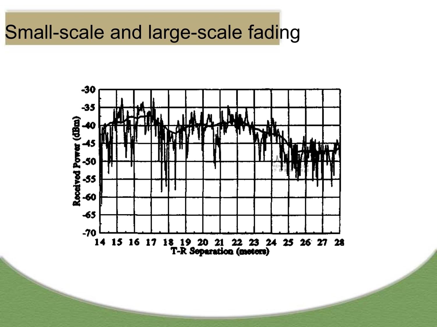
Propagation:Large-ScalePathLossSmall-scale

and

large-scale

fadingThe

three

Basic

Propagation

MechanismReflection:

occur

from

the

surface

of

the

earth

and

from

buildingsand

walls.Diffraction:occurs

when

the

radio

path

between

the

transmitterand

receiver

is

obstructed

by

a

surface

that

has

sharpirregularities(edges).Scattering:occurs

when

the

medium

through

which

the

wavetravels

consists

of

objects

with

dimensions

that

are

smallcompared

to

the

wavelength,

and

where

the

number

of

obstaclesper

unit

volume

islarge.SpectrumVLF

=

Very

Low

Frequency

,

LF

=

Low

Frequency

,

MF

=

Medium

Frequency

,HF

=

High

Frequency

,

VHF

=

Very

High

Frequency,

UHF

=

Ultra

HighFrequency,SHF

=

Super

High

Frequency,EHF

=

Extra

High

Frequency,UV

=

Ultraviolet

Light,Frequency

and

wave

length:

=

c/f

,wave

length

,

speed

of

light

c

3x108m/s,

frequencyf1

Mm300Hz10

km30

kHz100

m3

MHz1

m300MHz10

mm30

GHz100

m3

THz1

m300THzVLFLF

MF

HF

VHF

UHF

SHF

EHFinfraredvisible

light

UVoptical

transmissioncoax

cabletwistedpairFrequencies

for

mobile

communicationVHF-/UHF-ranges

for

mobileradiosimple,

small

antenna

for

carsdeterministic

propagation

characteristics,

reliableconnectionsSHF

and

higher

for

directed

radio

links,satellitecommunicationsmall

antenna,

focusinglarge

bandwidthavailableWireless

LANs

use

frequencies

in

UHF

to

SHF

spectrumFree

Space

Propagation

ModelIn

free

space,

the

received

power

is

predicted

byPr(d):

Received

power

with

a

distance

d

between

Tx

and

RxPt:

TransmittedpowerGt:

Transmitting

antenna

gainGr:

Receive

antennagain:

The

wavelength

in

meters.d:

distance

inmetersL:

The

miscellaneous

losses

L

(L>=1)

are

usually

due

to

transmission

lineattenuation,

filter

losses,

and

antenna

losses

in

the

communication

system.L=1

indicates

no

loss

in

the

system

hardware.EIRP&ERP2.15dBEIRP:

Effective

Isotropic

Radiated

PowerRepresents

the

maximum

radiated

power

available

from

a

transmitter

in

thedirection

of

maximum

antenna

gain,

as

compared

to

an

isotropic

radiator.ERP:

Effective

Radiated

PowerERP

is

used

instead

of

EIRP

to

denote

the

maximum

radiated

power

ascompared

to

ahalf-wave

dipole

antenna

(instead

of

an

isotropicantenna).In

practice,

antenna

gains

are

given

in

units

of

dBi

(dB

gain

with

respect

to

anisotropic

sourse)

or

dBd

(dB

gain

with

respect

to

ahalf-wavedipole)9dBi

antenna

&

3dBiantennaPath

LossThe

path

loss,

which

represents

signal

attenuation

as

a

positivedifference

(in

dB)

between

the

effective

transmitted

power

and

thereceived

power.

The

path

loss

for

the

free

space

model

when

antenna

gains

areincluded

is

given

by

quantity

measured

in

dB,

is

defined

as

theWhen

antenna

gains

are

excluded,

the

antennas

are

assumed

to

haveunity

gain,

and

path

loss

is

given

by(f:MHz,d:km)Thefar-field

region

of

a

transmitting

antennaThe

Friis

free

space

model

is

only

a

valid

predictor

for

Pr

for

values

ofd,

which

are

in

the

far-field

of

the

transmitting

antenna.The

far-field

of

a

transmitting

antenna

is

defined

as

the

region

beyondthe

far-field

distance

df

,

which

is

related

to

the

largest

lineardimensionof

the

transmitter

antenna

aperture

and

the

carrier

wavelength.

The

far-field

distance

is

given

byTo

be

inthe

far-field

region,dmust

satisfyThe

Reference

DistanceIt

is

clear

that

equation

does

not

hold

for

d=0.

For

this

reason,large-scale

propagation

models

use

a

known

received

powerreferencepoint.

The

received

power,

Pr(d),

at

any

distance

d>d0,

may

berelated

to

Pr

at

d0.If

Pr

is

in

units

ofdBm

or

dBW,

the

received

power

is

given

byLog-distance

pathlossmodelBoth

theoretical

andmeasurement-based

propagation

models

indicate

thataverage

received

signal

power

decreases

logarithmically

with

distance,whether

in

outdoor

or

indoor

channels.

The

average

large-scale

path

lossfor

an

arbitrary

T-R

separation

is

expressed

as

a

function

of

distance

byusing

path

loss

exponentn.n

is

the

path

loss

exponent

which

indicates

the

rate

at

which

the

path

lossincreases

with

distanced0

is

the

close-in

reference

distance

which

is

determinedd

is

the

T-R

separation

distanceIf

a

transmitter

produces

power:Pt=50w,

receive

sensitivity

(minimum

usablesignal

level)is

-100dbm.Assume

d0=100m,

with

a

900MHz

carrier

frequency,n=4,Gt=Gr=1;

find

the

coverage

distance

d.Transmit

Power:

Pt=50W=47dBmPr(d0)=-24.5dBmPL(dB)=40log(d/d0)=-24.5-(-100)=75.5dbmIfn=4,log(d/d0)=75.5/40=1.8875,d=7718mExampleLog-normal

ShadowingThe

model

in

Equation

(3.11)

does

not

consider

the

fact

that

thesurrounding

environmental

clutter

may

be

vastly

different

at

two

differentlocations

having

the

same

T-R

separation.

This

leads

to

measuredsignalswhich

are

vastly

different

than

the

average

value

predicted

byEquation(3.11).Simulation

ResultsDeep

shadowingSlight

ShadowingLog-normalShadowingDetermination

of

Percentage

of

Coverage

Areaas

a

function

of

probability

of

signal

above

threshold

on

the

cell

boundary.Example

Four

received

power

measurements

were

taken

at

distances

of

100

m,

200

m,1

km,

and

3

km

from

a

transmitter.

These

measured

values

are

given

in

the

followingtable.

It

is

assumed

that

the

path

loss

for

these

measurements

follows

the

model

inEquation(3.12.a),where

d0

=100

m:(a)

findtheminimummean

square

error(MMSE)estimate

for

the

path

loss

exponent,

n;

(b)

calculate

the

standard

deviation

about

themean

value;

(c)

estimate

the

received

power

at

d

=

2

km

using

the

resulting

model;

(d)predict

the

likelihood

that

the

received

signal

level

at

2

km

will

be

greater

than

-60dBm

;

and

(e)

predict

the

percentage

of

area

within

a

2

km

radius

cell

that

receivessignals

greater

than

-60dBm,

given

the

result

in

(d).The

value

of

n

which

minimizes

the

mean

square

error

can

be

obtained

byequating

the

derivative

of

J(n)

to

zero,

and

then

solving

for

n.(a)Using

Equation

(3.11),

we

find =

pi(d0)-10nlog(di/

100

m).

Recognizing

thatP(d0)

=

0

dBm,

we

find

the

following

estimates

for

p,

in

dBm:The

MMSE

estimate

may

be

found

using

the

following

method.

Let

pi

be

the

receivedpower

at

a

distance

di,

and

let be

the

estimate

for

pi

using

the path

lossmodel

of

Equation

(3.10).

The

sum

of

squared

errors

between

the

measured

andestimated

values

is

given

bySetting

this

equal

to

zero,

the

value

of

n

is

obtained

asn

=

4.4.(b)The

sample

variance

o2

=

J(n)/4

atn

=

4.4

can

be

obtained

asfollows.therefore=

6.17

dB,

which

is

a

biased

estimate.The

estimate

of

the

received

power

at

d

=

2

km

isThe

probability

that

the

received

signal

level

will

be

greater

than

-60dBm

is67.4%

of

the

users

on

the

boundary

receive

signals

greater

than-60

dBm,

then

92%

of

the

cell

area

receives

coverage

above–60dbmOutdoor

Propagation

ModelsOkumura

ModelHata

modelOkumura

Modelnot

provide

any

analytical

explanationits

slow

response

to

rapid

changes

interrainOkumura

median

attenuation

and

correctionFind

the

median

path

loss

using

Okumura's

model

for

d

=

50km,

hte

=

100

m,hre

=

10

m

in

a

suburban

environment.

If

thebase

station

transmitter

radiates

an

EIRP

of

1

kW

at

acarrierfrequency

of

900

MHz,

find

the

power

at

thereceiver(assume

a

unity

gain

receivingantenna).Example

3HATA

model

&COST

–231extensionExample

4In

the

suburban

of

a

large

city,

d

=

10

km,

hte

=

200

m,

hre

=2

m

,

carrier

frequency

of

900

MHz,

using

HATA’

smodelfind

the

path

loss.Indoor

propagation

modelsFeature

of

Indoor

Radio

ChannelThe

distances

covered

are

much

smaller,

and

the

variabilityof

the

environment

is

much

greater

for

a

much

smallerrangeof

T-R

separation

distances.

It

has

been

observed

thatpropagation

within

buildings

is

strongly

influenced

byspecific

features

such

as

the

layout

of

the

building,

theconstruction

materials,

and

the

building

type.Indoor

radio

propagation

is

dominated

by

the

samemechanisms

as

outdoor:

reflection,

diffraction,

and

scattering.However,

conditions

are

much

more

variable.Path

attenuation

factorsDistance

LossesPartition

Losses

in

the

same

floorPartition

Losses

between

Floors(floor

attenuationfactors,

FAF)Log-distance

Path

LossModelIn

door

path

loss

has

been

shown

by

many

researchersto

obey

the

distance

power

lawWhere

the

value

of

n

depends

on

the

surroundings

andbuilding

type,and

X

represents

a

normal

randomvariable

in

dB

having

a

standard

deviation

of

sigma.

Thisis

identical

in

form

to

thelog-normal

shadowing

model

ofoutdoor

path

attenuation

model.Attenuation

Factor

ModelWhere

nSF

represents

the

exponent

value

for

the

“same

floor”measurement. The

path

loss

on

a

different

floor

can

bepredicted

by

adding

an

appropriate

value

of

FAFSignal

Penetration

into

buildingsRF

penetration

has

been

found

to

be

a

function

of

frequency

aswell

as

height

within

the

buildingMeasurements

showed

that

penetration

loss

decreases

withincreasing

frequency.

Specifically,

penetration

attenuationvalues

of

16.4dB,

11.6dB,and

7.6dB

were

measured

on

theground

floor

of

a

building

at

frequencies

of

441MHz,896.5MHz,

and

1400Mhz,respectly.Results

showed

that

building

penetration

loss

decreased

at

arateof

1.9dB

per

floor

from

the

ground

level

up

to

the

fifteenth

floorand

then

began

increasing

above

the

fifteenfloor.Ray

Tracing

and

Site

Specific

ModelingIn

recent

years,

the

computational

and

visualization

capabilities

of

computers

haveaccelerated

rapidly.

New

methods

for

predicting

radio

signal

coverage

involve

theuse

of

Site

Specific

(SISP)

propagation

models

and

graphical

informationsystem(GIS)

database.

SISP

models

support

ray

tracing

as

a

means

ofdeterministicallymodeling

any

indoor

or

outdoor

propagation

environment.

Through

the

use

ofbuilding

databases,

which

may

be

drawn

or

digitized

using

standardgraphicalsoftware

packages,

wireless

system

designers

are

able

to

include

accuraterepresentations

of

building

and

terrain

features.ExercisesIf

a

transmitter

produces

50W

of

power,

express

the

transmit

power

inunits

of

(a)dBm,

and

(b)

dBW.

If

50