pid简介及英语翻译

1、PID ControlIntroductionThe PID controller is the most common form of feedback. It was an essential element of early governors and it became the standard tool when process control emerged in the 1940s. In process control today, more than 95% of the control loops are of PID type, most loops are actual

2、ly PI control. PID controllers are today found in all areas where control is used. The controllers come in many different forms. There are standalone systems in boxes for one or a few loops, which are manufactured by the hundred thousands yearly. PID control is an important ingredient of a distribut

3、ed control system. The controllers are also embedded in many special purpose control systems. PID control is often combined with logic, sequential functions, selectors, and simple function blocks to build the complicated automation systems used for energy production, transportation, and manufacturin

4、g. Many sophisticated control strategies, such as model predictive control, are also organized hierarchically. PID control is used at the lowest level; the multivariable controller gives the set points to the controllers at the lower level. The PID controller can thus be said to be the “bread and bu

5、tter of control engineering. It is an important component in every control engineers tool box.PID controllers have survived many changes in technology, from mechanics and pneumatics to microprocessors via electronic tubes, transistors, integrated circuits. The microprocessor has had a dramatic influ

6、ence the PID controller. Practically all PID controllers made today are based on microprocessors. This has given opportunities to provide additional features like automatic tuning, gain scheduling, and continuous adaptation.The AlgorithmWe will start by summarizing the key features of the PID contro

7、ller. The “textbook” version of the PID algorithm is described by: 6.1where y is the measured process variable, r the reference variable, u is the control signal and e is the control error（e = y）. The reference variable is often called the set point. The control signal is thus a sum of three terms:

8、the P-term （which is proportional to the error）, the I-term （which is proportional to the integral of the error）, and the D-term （which is proportional to the derivative of the error）. The controller parameters are proportional gain K, integral time Ti, and derivative time Td. The integral, proporti

9、onal and derivative part can be interpreted as control actions based on the past, the present and the future as is illustrated in Figure 2.2. The derivative part can also be interpreted as prediction by linear extrapolation as is illustrated in Figure 2.2. The action of the different terms can be il

10、lustrated by the following figures which show the response to step changes in the reference value in a typical case.Effects of Proportional, Integral and Derivative ActionProportional control is illustrated in Figure 6.1. The controller is given by D6.1E with Ti = and Td=0. The figure shows that the

11、re is always a steady state error in proportional control. The error will decrease with increasing gain, but the tendency towards oscillation will also increase.Figure 6.2 illustrates the effects of adding integral. It follows from D6.1E that the strength of integral action increases with decreasing

12、 integral time Ti. The figure shows that the steady state error disappears when integral action is used. Compare with the discussion of the “magic of integral action” in Section 2.2. The tendency for oscillation also increases with decreasing Ti. The properties of derivative action are illustrated i

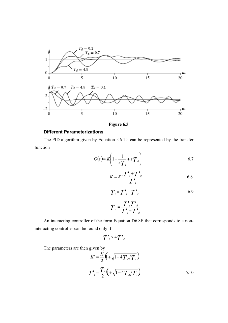
13、n Figure 6.3.Figure 6.3 illustrates the effects of adding derivative action. The parameters K and Ti are chosen so that the closed loop system is oscillatory. Damping increases with increasing derivative time, but decreases again when derivative time becomes too large. Recall that derivative action

14、can be interpreted as providing prediction by linear extrapolation over the time Td. Using this interpretation it is easy to understand that derivative action does not help if the prediction time Td is too large. In Figure 6.3 the period of oscillation is about 6 s for the system without derivative

15、Chapter 6. PID ControlFigure 6.1Figure 6.2Derivative actions cease to be effective when Td is larger than a 1 s (one sixth of the period). Also notice that the period of oscillation increases when derivative time is increased.There is much more to PID than is revealed by （6.1）. A faithful implementa

16、tion of the equation will actually not result in a good controller. To obtain a good PID controller it is also necessary to consider。Figure 6.3Different ParameterizationsThe PID algorithm given by Equation（6.1）can be represented by the transfer function 6.7 6.8 6.9 An interacting controller of the f

17、orm Equation D6.8E that corresponds to a non-interacting controller can be found only ifThe parameters are then given by 6.10The non-interacting controller given by Equation （6.7） is more general, and we will use that in the future. It is, however, sometimes claimed that the interacting controller i

18、s easier to tune manually.It is important to keep in mind that different controllers may have different structures when working with PID controllers. If a controller is replaced by another type of controller, the controller parameters may have to be changed. The interacting and the non-interacting f

19、orms differ only when both I and the D parts of the controller are used. If we only use the controller as a P, PI, or PD controller, the two forms are equivalent. Yet another representation of the PID algorithm is given by 6.11The parameters are related to the parameters of standard form through The

20、 representation Equation （6.11） is equivalent to the standard form, but the parameter values are quite different. This may cause great difficulties for anyone who is not aware of the differences, particularly if parameter 1/ki is called integral time and kd derivative time. It is even more confusing

21、 if ki is called integration time. The form given by Equation （6.11） is often useful in analytical calculations because the parameters appear linearly. The representation also has the advantage that it is possible to obtain pure proportional, integral, or derivative action by finite values of the pa

22、rameters.PID介绍PID控制器是反馈控制的最常见形式。因为早在40年代它就成为了过程控制的标准工具。在今天的过程控制业中，超过95%的控制回路是PID类型，多数实际上是PI 控制。PID控制是分布控制系统的一种重要组成部分。控制器被隐藏在许多其他控制系统下面。PID 控制与逻辑控制经常结合在一起,连续作用、选择器，和简单的功能模块一起构成复杂自动化系统，可以应用在发电、运输，以及制造业。许多经典的控制策略，譬如模型有预测性的控制。PID控制是使用在要求水平较低的场合；PID控制器应用在底层。PID控制器在每个控制工程师的应用实例里都能经常见到。近年来PID控制器在技术生产上也产生了许

23、多变化，从机械到微处理器控制由电子管，晶体管,组合电路组成的控制系统。微处理器对PID控制器有着强烈的影响。实际上今天制作的所有PID控制器都是建立在微处理器的基础上的。这就有机会扩展其他的特点：像自动定调，获取预定，和连续的适应。6.2 算法我们开始讲解PID控制器的主要特点。 PID算法的描述： 6.1这里 y 是被测量的处理可变量, r 参考可变量, u 是控制信号，e是控制误差 。参考变量经常可以被称为是固定的点。控制信号包含三个量，P-term，I-term，D-term，控制器的参数包括比例系数K，整体时间Ti，和Td。以过去，现在和未来为基础的控制轨迹可解释整体，比例项和输出部份的关系。图中举例。在不同时间的运动可以表示输出部分的一个典型的例子。在参数值方面作一下改变，即可预测下一时间的走向问题。PID的作用图6.1说明的是典型的比例控制。控制器给定Ti=，Td=0。表示在比例控制中总存在有一种稳定状态误差。获取值增加误差将减少，但系统稳定性将受到影响。图 6.2 说明增加积分式的作用。它跟随图6.1而来增加时间Ti.当积分式运行使用。稳定状态误差将逐渐的